5.9.2 Negative Binomial
The command used to run a Negative Binomial analysis is negative-binomial.
The first variable in the list is the dependent variable (counting variable that counts occurrences of a given event). Other variables (explanatory variables) can be specified in the same way as with OLS (cf. the regress command).
Available options:
-
noconstant: Suppresses the constant term -
level(): Change from default 95% confidence interval -
robust: Robust standard errors -
cluster(): Use cluster variable (cannot be used together with robust) -
control(): Do not show coefficient estimates for selected variables -
irr: Reports incidence rate ratio values instead of coefficient values (the values are transformed through the natural exponential function). The value 1 means no effect. Values above 1 mean a positive effect, while values below 1 mean a negative effect. -
exposure(): Includes exposure variable. This represents the amount of exposure to the process that generates counts. The variable entered inside the parentheses is usually continuous and must not contain 0 values. For example, if you are modeling the number of car accidents in different cities, the number of residents in each city can be an exposure variable. Typically, a variable is used that can be used to calculate rates for the count in question. The exposure variable is automatically log-transformed (natural logarithm) and included as an offset in the model, meaning it will adjust the count response for the amount of exposure. The other estimates are then corrected based on this variable, so that they become more correct. Note that theexposurevariable should not be entered as an explanatory variable in the model.
Factor variables, and cluster and robust estimation can also be used. The procedure is the same as for ordinary linear regression. See respectively chapter 5.4.1 and 5.4.3 for more information on this. For a full list of possibilities, use the help negative-binomial command.
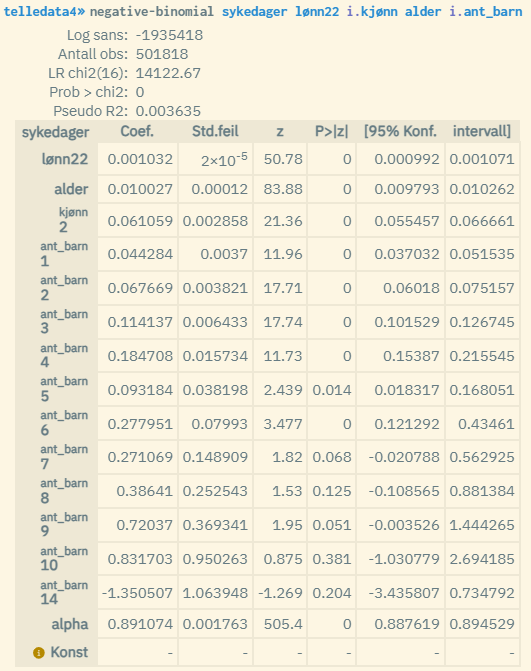
Example of Negative Binomial Regression:

Note that the implementation of the counter regression Negative Binomial in microdata.no is not compatible with statistical models where at least one of the explanatory variables has too high a value (this will typically apply to income variables). It is recommended to transform the values of the relevant variables so that they fall below a limit value of approx. 400 (this can be done by dividing by a factor or using e.g. a logarithm transformation). If this is not done, you risk getting a result that only shows empty values. However, as long as estimates are reported for all the explanatory variables, you do not need to perform any transformation.
Negative Binomial vs. Poisson
The difference between a Poisson regression and a Negative Binomial regression is that in the latter the parameter alpha is included to capture extra variance (overdispersion), and the value of this is reported at the bottom of the list of coefficient estimates (above the constant term). The parameter is thus used to scale the variance of the model1.
An alpha value of 0 means that the model is identical to a Poisson model where variance = mean for the response variable, and that a Poisson regression is more appropriate to use. Positive alpha values indicate overdispersion (greater spread), and the higher the value, the greater the spread. In the example above, the value is 0.89. This suggests that there is a relatively large degree of overdispersion and that Negative Binomial regression is possibly best to use (although Pseudo R2 has a lower value compared to Poisson).
Source:
The algorithms for the negative-binomial command are based on the function NegativeBinomial found in the Statsmodels module in Python.
Footnote:
Footnotes
-
The variance of a Negative Binomial model can be expressed as follows: Variance = μ + α * μ2 , where μ = average of Y, α = alpha. In a Poisson model, alpha is equal to 0 so that variance = mean. ↩